Hi!

I'm Isha

And I’m a Chartered Accountant. I love Teaching, Mentoring and Hustling, while having coffee with my pet Sherry.

TAX SAVING | EXCEL | POWER POINT | POWER BI | TABLEAU | CAREER GUIDANCE | INTERVIEW TIPS | CORPORATE TRAININGS | TAX SAVING | EXCEL | POWER POINT | POWER BI | TABLEAU | CAREER GUIDANCE | INTERVIEW TIPS | CORPORATE TRAININGS |

Get More Free Tips Delivered Straight to Your Inbox

Book your seat in my upcoming Excel Masterclass (Dates to be announced soon)

Guide on 3 New Excel Formulas

SEQUENCE

Generates a sequence of numbers in an array, allowing customization of the start value, end value, step size, and array dimensions.

Formula Layout:

=SEQUENCE(rows, [columns], [start], [step])

  • rows: Number of rows in the sequence.
  • [columns] (optional): Number of columns in the sequence. If omitted, defaults to 1.
  • [start] (optional): Starting value of the sequence. If omitted, defaults to 1.
  • [step] (optional): Step size between each value in the sequence. If omitted, defaults to 1.


Example:

=SEQUENCE(5) // Generates a sequence of 5 numbers starting from 1

=SEQUENCE(3, 4, 10, 5) // Generates a 3×4 array starting from 10 with a step size of 5


Here’s an alternate way to add numbering in Excel:

https://www.instagram.com/reel/C0G539xSCfH/?igsh=YnA0aWUwNWptZjgz

UNIQUE

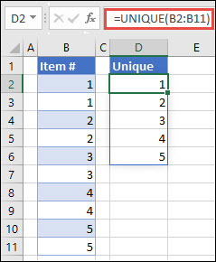
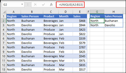
Returns a list of unique values from a range or array, eliminating duplicates and simplifying data analysis and reporting tasks.

Formula Layout:

=UNIQUE(array, [by_col], [exactly_once])

  • array: The range or array from which you want to extract unique values
  • [by_col] (optional): TRUE if you want to compare values by columns, FALSE or omitted if by rows
  • [exactly_once] (optional): TRUE to return only values that appear exactly once, FALSE or omitted to return all unique values.


Example:

=UNIQUE(B2:B11) – Returns a list of unique values from cells A1 to A10

Example of using =UNIQUE(B2:B11) to return a unique list of numbers

=UNIQUE(A2:B13) – Returns unique values comparing by columns in the range A2:B13

Using UNIQUE to return a list of sales people.

XMATCH

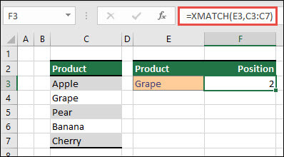
Finds and returns the relative position of a specified item in a range or array, providing more flexibility than traditional lookup functions by supporting approximate and exact matches, as well as searching in any direction.

Formula Layout:

=XMATCH(lookup_value, lookup_array, [match_type], [search_mode])

  • lookup_value: The value you want to find in the lookup_array.
  • lookup_array: The range or array where you want to search for the lookup_value
  • [match_type] (optional): Specifies the type of match to perform:
    • 0 or omitted: Exact match (default).
    • -1: Exact match or next smallest value.
    • 1: Exact match or next largest value.
    • 2: Wildcard characters are allowed in lookup_value. (This requires lookup_array to be sorted.)
  • [search_mode] (optional): Specifies the search mode:
    • 1 or omitted: Search first to last.
    • -1: Search last to first.


Example:

=XMATCH(E3, C3:C7, 0, 1) –

This formula would search for the value in cell E3 within the range C3:C7 and return the relative position of the first exact match, searching from first to last.

Example of using XMATCH to find the position of an item in a list

Get More Free Tips Delivered Straight to Your Inbox

Book your seat in my upcoming Excel Masterclass (Dates to be announced soon)